As part of my internship I designed and wrote code to analyze a person’s movements for a security app for cellphones. This application is supposed to track a persons movements in real time and compare the data to a model and schedule that was generated from previous observations. If there are any anomalies between the two data sets, it will have to determine if the deviation was caused by a change in the schedule, or because the person in question is in trouble and needs help.
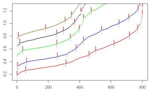
One algorithm that is being used is a Segmented Least Squares. The data that is collected from the smart phone gets cleaned up, filtered, and converted into a two dimensional time series graph. This data is then segmented by the algorithm and a best fit graph is produced. The resulting graph is determined by a particular input variable called the penalty factor that can be changed by the user (see below for more details), so results can very between runs. The information gathered can be written to an XML file. Several Java classes have been created for this and thoroughly tested with JUnit.
For those unfamiliar with Segmented Least Squares, it is a type of linear regression algorithm. Using an equation to calculate the amount of error produced, this algorithm comes up with the best possible fit for a data set. The error is calculated based off of how many line segments are used and the sum of the error produced between each data point and its predicted value (which is determined by the line segments).
The main issue with this algorithm is the penalty factor that is added in to the total error each time you start a new segment. While this isn’t as big an issue with test data that contains little to no noise, when it comes to real world data (which usually contains lots of noise) it is difficult to find the ‘right’ penalty factor, so the end result will always be slightly off from the desired outcome.
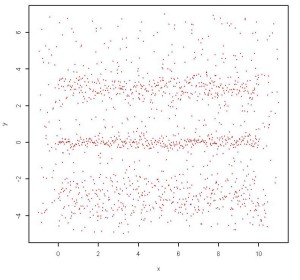
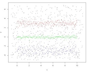
Another algorithm that is being used is a cluster algorithm. This is so that the program can recognize which data points represent what, by checking to see which cluster node it is closest to. While this is a great method for classifying, the one issue with it is that you need to set the number of clusters before running this algorithm (unless you choose a density based clustering algorithm, which has its own downfalls). However, that isn’t that big a problem if you already know what groups you are representing. Also if you already know what the data points will look like for each cluster, then identification won’t be an issue.
Clustering is the grouping of a set of objects in such a way that objects in the same group are more similar to each other than to those in other groups. It is used in data mining and common in data analysis. It is also used in many fields such as machine learning, pattern recognition, information retrieval, image analysis. There are different types of clustering algorithms that will all produce different results.
The two most well know cluster types are K Means and Density based. K means requires the user to input the number of clusters they want. The results of the K Means should be mostly the same for each run if using the same cluster number with the same data set, but there will most likely be some points that will jump between some of the clusters because of their border line location. Density Based is as the name is implied: the clusters are determined by the densities in the data set. The result could be different from what the user predicted since with Density Based and you can wind up with a cluster within a cluster.
The project also implements a Hidden Markov Model. A basic Markov Model uses probability to predict what the next state you will enter based on what your current state is. The state is directly visible to the observer, and therefore the state transition probabilities are the only parameters. In a Hidden MM, the state is not directly visible, but output, dependent on the state, is visible. Each state has a probability distribution over the possible output tokens. Therefore the sequence of tokens generated by an HMM gives some information about the sequence of states. It should be made clear that the ‘hidden’ part of HMM refers to the state sequence through which the model passes, not to the parameters of the model.


